Seasonal and monthly models • hydroState

library(hydroState)

Sub-annual models

Seasonal and monthly models provide further insight into the state of the rainfall-runoff relationship throughout the year, but with this more sensitive analysis, there is often more seasonal variation and auto-correlation. hydroState provides additional options to explain this variation so models are statistically adequate. These options are located within the build() function. The seasonal variation can be explained with a sinusoidal function for a particular parameter through identifying seasonal.parameters in build(). This vignette provides an example of an analysis on a seasonal time-step with the intercept, a0, as a seasonal.parameters.

Load required data

Seasonal and monthly rainfall-runoff models require a data frame with catchment average runoff and precipitation for each month. Load the data into the environment. Ensure there are four columns named “year”, “month”, “flow”, and “precipitation”, and verify the units for flow and precipitation are the same (‘mm’, ‘in’, etc.).

Note, hydroState parses the input.data given in sequential order by year, month, and day (1950-01-01, 1950-01-02 or 1978-11, 1978-12, 1980-01, etc). Avoid re-labeling months in water-years for seasonal and monthly input.data. Use calender years.

data(streamflow_monthly_415201)

# check input data
head(streamflow_monthly_415201)
#>   year month     flow precipitation
#> 1 1950     1 0.000000      2.316268
#> 2 1950     2 0.000000     86.074245
#> 3 1950     3 2.044923     58.934578
#> 4 1950     4 1.189653     40.083532
#> 5 1950     5 1.098197     82.928550
#> 6 1950     6 2.417402     20.966111

For a seasonal analysis, hydroState provides an additional get.seasons() function to adjust the monthly data into seasons. The flow and precipitation are summed every three months and shown in the last month of the season. The number of months in each season is included. An example of this is shown below.

# aggregate monthly data to seasonal
streamflow_seasonal_415201 = get.seasons(streamflow_monthly_415201)

# check seasonal data
head(streamflow_seasonal_415201)
#>   year month      flow precipitation nmonths
#> 1 1950     5  4.332774      181.9467       3
#> 2 1950     8  6.924973      126.3109       3
#> 3 1950    11  7.729439      170.7257       3
#> 4 1951     2  7.049185      141.9339       3
#> 5 1951     5  1.395975      128.1353       3
#> 6 1951     8 36.430009      227.4161       3

Build a sub-annual hydroState model

For seasonal and monthly models, there are additional options when building a model. A default model can be built that is identical to the default annual model except on a monthly or seasonal time-step OR the model can be adjusted.

In addition to the options presented in adjusting the default state model vignette, the seasonal and monthly models can assume parameters within the rainfall-runoff relationship vary seasonally throughout the year. This is available within the seasonal.parameters. This assumes a parameter is best modeled as a sinusoidal function representing seasonal trends. The input accepts any default parameter: a1, a0, or std. Typically, assuming seasonal trends in only the intercept, a0, explains trends in the residuals of the model. For further details, see build().

For this analysis, an adjusted model is built on a seasonal time-step:

# Build seasonal hydroState model with adjusted model, seasonal forcing
model.seasonal.adjusted = build(input.data = streamflow_seasonal_415201,
                          parameters = c('a0','a1','std','AR2'),
                          seasonal.parameters = 'a0',
                          data.transform = 'boxcox',
                          transition.graph = matrix(TRUE,3,3))

Fit the model

Fit the built models with fit.hydroState(). This will take typically an hour to run.

<!-- model.seasonal.adjusted = fit.hydroState(model.seasonal.adjusted, pop.size.perParameter = 10, max.generations = 10000, doParallel = TRUE)  -->

Review the residuals

Review the model’s residuals from figures using plot.hydroState() to ensure they are uniform and normally distributed with no trends or auto-correlation.

# review residual plots
plot(model.seasonal.fitted.415201, pse.residuals = TRUE, siteID = '415201'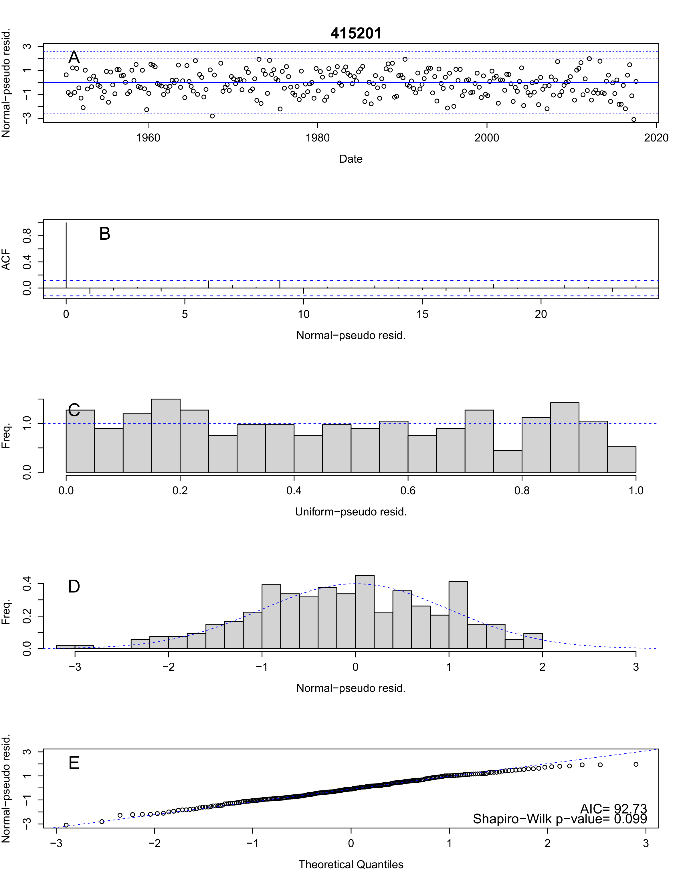, do.pdf = FALSE)

The residual plots of the best seasonal model for site 415201 are uniform and normally distributed with the Shapiro-Wilk p-value being greater than 0.05.

Evaluate the state-shifts

Set the state names relative to a year in the record using setInitialYear(). This provides a name for the states so they are easier to interpret in the following figures. Then plot the state-shifts overtime using plot.hydroState(). In this example, 1990 is chosen as the year of reference. All four plots within the function are shown here, but either plot or combination of plots can be selected. Alternatively, the states can be reviewed without plotting using get.states() which returns a data frame of states at each time-step.

# set the reference year to name the states
model.seasonal.fitted.415201 = setInitialYear(model.seasonal.fitted.415201, 1990)


# plot all four plots
plot(model.seasonal.fitted.415201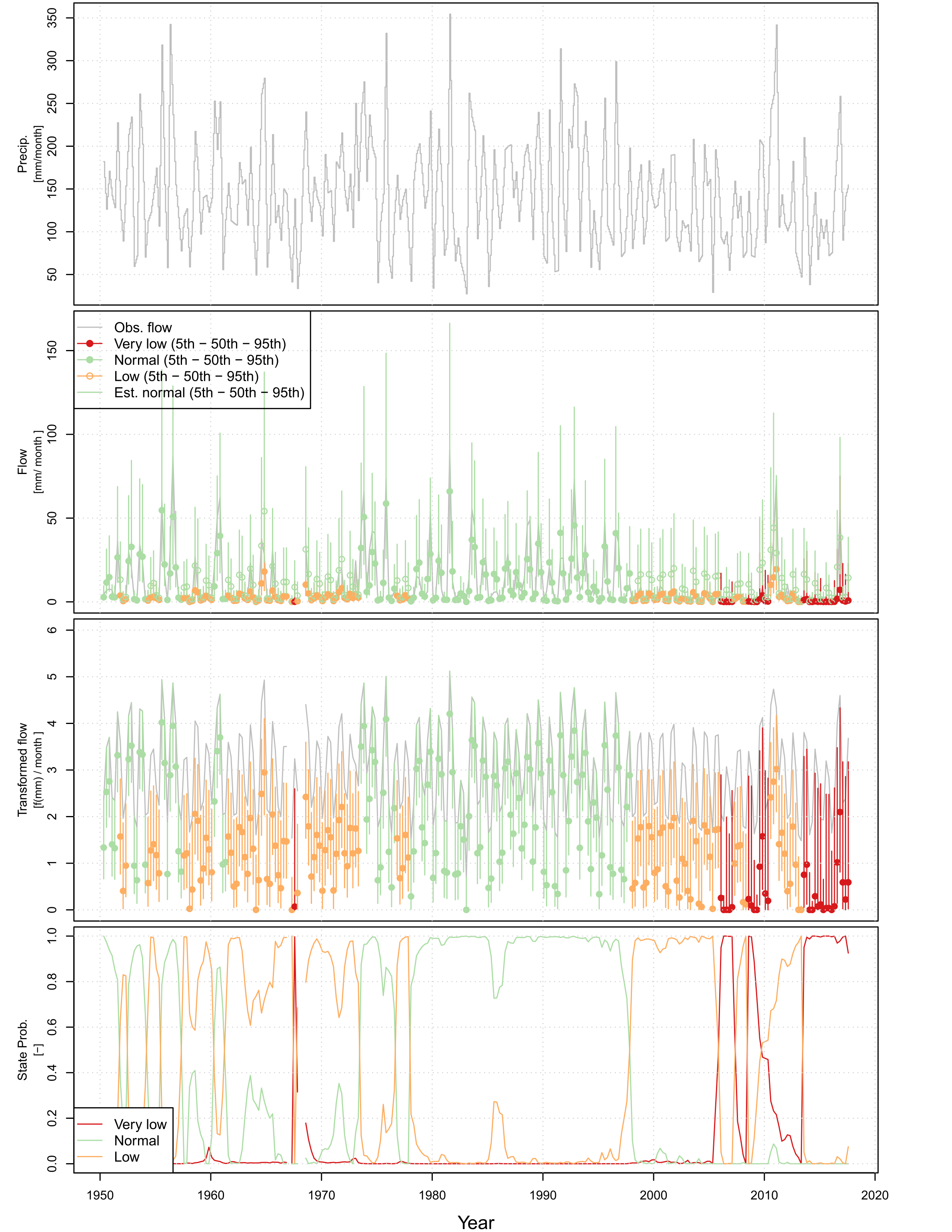, do.pdf = F)

The seasonal model considers seasonality and auto-correlation within the rainfall-runoff relationship, but these model results show there are state shifts within this relationship at this site. The 3-states suggests a shift in the rainfall-runoff relationship throughout the record better represent observations. The Very Low state persist at the end of the record after a prolonged drought from roughly 1997-2009.

Systematic model selection for sub-annual models

To identify the best sub-annual model, a systematic evaluation of the possible model combinations can be performed using the build.all() function. Below is an example evaluating all possible model combinations when a0 and std are the state dependent parameters, and a0 is expressed as a seasonal.parameter. The procedure is identical to the systematic model evaluation within the “Adjust the default state model vignette”, expect seasonal.parameters may be selected. Note, it is recommend to run this systematic analysis in parallel and on a high-performance computer where possible. The example below can take hours to fit 12 models when running in parallel on a 7-core, 64-bit operating system.

# Build all possible models with the intercept, 'a0', as a seasonal parameter and state dependent parameter
all.models.seasonal = build.all(input.data = streamflow_seasonal_415201,
                                        state.shift.parameter = c('a0','std'),
                                        seasonal.parameter = 'a0')

# Review the order of the reference models, adjust reference models if needed.
all.models.ref.table = summary(all.models.seasonal)

# Re-build with adjusted reference table
all.models.seasonal = build.all(input.data = streamflow_seasonal_415201,
                                        state.shift.parameter = c('a0','std'),
                                        seasonal.parameter = 'a0',
                                        summary.table = all.models.ref.table)

# Fit all models (takes hours to run)
<!-- all.models.seasonal = fit.hydroState(all.models.seasonal, pop.size.perParameter = 10, max.generations = 10000, doParallel = T) -->

# Identify the best model with the lowest AIC
get.AIC(all.models.seasonal.fitted.415201)

#>                                                  AIC    nParameters   AIC.weights
#> model.3State.gamma.boxcox.AR2.a0.seasonal.a0std  92.73299          23 9.999948e-01
#> model.3State.gamma.boxcox.AR3.a0.seasonal.a0std 117.07896          24 5.168178e-06
#> model.2State.gamma.boxcox.AR3.a0.seasonal.a0std 133.67572          15 1.286464e-09
#> model.3State.gamma.boxcox.AR1.a0.seasonal.a0std 150.25432          22 3.231464e-13
#> ...